Digit recognizer

Recognizing handwritten digits with a convolutional neural network.

Python
PyTorch
Author

Robbin Romijnders

Published

November 17, 2021

Abstract

The problem with handwritten digits.

Code
import numpy as np
import matplotlib.pyplot as plt
import torch
import torch.nn as nn
import torch.nn.functional as F
import torch.optim as optim
from torch.utils.data import DataLoader
import torchvision
from torchvision import datasets, transforms

# Define the data transforms
data_transforms = transforms.Compose([
    transforms.ToTensor(),
    transforms.Normalize(mean=(0.1307,), std=(0.3081,))
])

# Get the MNIST dataset
ROOT_PATH = "~/Datasets/PyTorch"
train_dataset = torchvision.datasets.MNIST(root=ROOT_PATH, train=True, transform=data_transforms, download=True)
test_dataset = torchvision.datasets.MNIST(root=ROOT_PATH, train=False, transform=data_transforms, download=True)

# Define the dataloaders
BATCH_SIZE = 64
train_loader = DataLoader(train_dataset, batch_size=BATCH_SIZE, shuffle=True)
test_loader = DataLoader(test_dataset, batch_size=BATCH_SIZE, shuffle=False)

# Visualize images
for example_images, example_labels in train_loader:
    break
num_cols = 8
num_rows = int(example_images.shape[0] // num_cols)
fig, axs = plt.subplots(num_rows, num_cols, figsize=(5, 5))
fig.subplots_adjust(wspace=0.05, hspace=0.05)
for example_idx in range(example_images.shape[0]):
    ax = axs[example_idx % num_cols, example_idx // num_cols]
    ax.imshow(example_images[example_idx].squeeze(), cmap="gray")
    ax.axis("off")
# plt.tight_layout()
plt.show()
0.3%0.7%1.0%1.3%1.7%2.0%2.3%2.6%3.0%3.3%3.6%4.0%4.3%4.6%5.0%5.3%5.6%6.0%6.3%6.6%6.9%7.3%7.6%7.9%8.3%8.6%8.9%9.3%9.6%9.9%10.2%10.6%10.9%11.2%11.6%11.9%12.2%12.6%12.9%13.2%13.6%13.9%14.2%14.5%14.9%15.2%15.5%15.9%16.2%16.5%16.9%17.2%17.5%17.9%18.2%18.5%18.8%19.2%19.5%19.8%20.2%20.5%20.8%21.2%21.5%21.8%22.1%22.5%22.8%23.1%23.5%23.8%24.1%24.5%24.8%25.1%25.5%25.8%26.1%26.4%26.8%27.1%27.4%27.8%28.1%28.4%28.8%29.1%29.4%29.8%30.1%30.4%30.7%31.1%31.4%31.7%32.1%32.4%32.7%33.1%33.4%33.7%34.0%34.4%34.7%35.0%35.4%35.7%36.0%36.4%36.7%37.0%37.4%37.7%38.0%38.3%38.7%39.0%39.3%39.7%40.0%40.3%40.7%41.0%41.3%41.7%42.0%42.3%42.6%43.0%43.3%43.6%44.0%44.3%44.6%45.0%45.3%45.6%45.9%46.3%46.6%46.9%47.3%47.6%47.9%48.3%48.6%48.9%49.3%49.6%49.9%50.2%50.6%50.9%51.2%51.6%51.9%52.2%52.6%52.9%53.2%53.6%53.9%54.2%54.5%54.9%55.2%55.5%55.9%56.2%56.5%56.9%57.2%57.5%57.9%58.2%58.5%58.8%59.2%59.5%59.8%60.2%60.5%60.8%61.2%61.5%61.8%62.1%62.5%62.8%63.1%63.5%63.8%64.1%64.5%64.8%65.1%65.5%65.8%66.1%66.4%66.8%67.1%67.4%67.8%68.1%68.4%68.8%69.1%69.4%69.8%70.1%70.4%70.7%71.1%71.4%71.7%72.1%72.4%72.7%73.1%73.4%73.7%74.0%74.4%74.7%75.0%75.4%75.7%76.0%76.4%76.7%77.0%77.4%77.7%78.0%78.3%78.7%79.0%79.3%79.7%80.0%80.3%80.7%81.0%81.3%81.7%82.0%82.3%82.6%83.0%83.3%83.6%84.0%84.3%84.6%85.0%85.3%85.6%85.9%86.3%86.6%86.9%87.3%87.6%87.9%88.3%88.6%88.9%89.3%89.6%89.9%90.2%90.6%90.9%91.2%91.6%91.9%92.2%92.6%92.9%93.2%93.6%93.9%94.2%94.5%94.9%95.2%95.5%95.9%96.2%96.5%96.9%97.2%97.5%97.9%98.2%98.5%98.8%99.2%99.5%99.8%100.0%
100.0%
2.0%4.0%6.0%7.9%9.9%11.9%13.9%15.9%17.9%19.9%21.9%23.8%25.8%27.8%29.8%31.8%33.8%35.8%37.8%39.7%41.7%43.7%45.7%47.7%49.7%51.7%53.7%55.6%57.6%59.6%61.6%63.6%65.6%67.6%69.6%71.5%73.5%75.5%77.5%79.5%81.5%83.5%85.5%87.4%89.4%91.4%93.4%95.4%97.4%99.4%100.0%
100.0%
Figure 1: A batch of example images of handwritten digits.

Build a model

We start off with building a baseline model that simply takes all individual pixels and passes them through a fully connected network.

Code
class BaselineModel(nn.Module):
    def __init__(self):
        super().__init__()

        self.flatten = nn.Flatten()
        self.linear1 = nn.Linear(in_features=28 * 28, out_features=16)
        self.linear2 = nn.Linear(in_features=16, out_features=10)

    def forward(self, x):
        x = self.flatten(x)
        x = F.relu(self.linear1(x))
        x = self.linear2(x)
        return x

Train the model

In PyTorch we need to make sure that the model and data live on the same device. Obviously, if we can use a GPU to speed up the training, we would do this. Therefore, we first check for the device, and then move the model and data there.

Code
device = torch.device("cuda" if torch.cuda.is_available() else "cpu")

# Create an instance of the model
baseline_model = BaselineModel().to(device)

# Define the loss function to use
loss_fn = nn.CrossEntropyLoss()

# Use a common optimizer
optimizer = optim.Adam(baseline_model.parameters(), lr=0.001)

We define a separate function for validation that we can call after each training epoch:

Code
def eval_step(
    model: nn.Module,
    dataloader: DataLoader,
    loss_fn: nn.Module,
    device: torch.device
):
    # Put the model in eval mode
    model.eval()

    # Initialize performance metrics
    running_loss = 0.0
    correct = 0
    total = 0

    with torch.no_grad():
        for features, targets in dataloader:
            # Put the data and target to the device
            features, targets = features.to(device), targets.to(device)

            # Make predictions -- forward propagation
            predictions = model(features)

            # Calculate the loss
            loss = loss_fn(predictions, targets)

            # Track progress
            running_loss += loss.item()
            _, predicted = torch.max(predictions, 1)
            total += targets.size(0)
            correct += (predicted == targets).sum().item()

    avg_loss = running_loss / len(dataloader)
    accuracy = 100. * correct / total
    return avg_loss, accuracy

def train_step(
    model: nn.Module,
    dataloader: DataLoader,
    loss_fn: nn.Module,
    optimizer: optim.Optimizer,
    device: torch.device
):
    # Put the model in training mode
    model.train()

    # Initialize performance metrics
    running_loss = 0.0
    correct = 0
    total = 0

    for batch_idx, (features, targets) in enumerate(dataloader):
        # Put the data and targets to the correct device
        features, targets = features.to(device), targets.to(device)

        # Reset the optimizer
        optimizer.zero_grad()

        # Make predictions
        predictions = model(features)

        # Calculate the loss
        loss = loss_fn(predictions, targets)

        # Calculate the adjustments
        loss.backward()
        
        # Update the model
        optimizer.step()

        # Track progress
        running_loss += loss.item()
        _, predicted = torch.max(predictions, 1)
        total += targets.size(0)
        correct += (predicted == targets).sum().item()
    
    average_loss = running_loss / len(dataloader)
    accuracy = 100. * correct / total
    return average_loss, accuracy

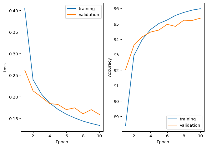
Now train the model for several epochs on the training data, and after each epoch get the validation loss and accuracy.

Code
NUM_EPOCHS = 10

history = {metric: [] for metric in ["train_loss", "train_acc", "val_loss", "val_acc"]}

for epoch in range(NUM_EPOCHS):
    train_loss, train_acc = train_step(model=baseline_model, dataloader=train_loader, loss_fn=loss_fn, optimizer=optimizer, device=device)
    val_loss, val_acc = eval_step(model=baseline_model, dataloader=test_loader, loss_fn=loss_fn, device=device)
    history["train_loss"].append(train_loss)
    history["train_acc"].append(train_acc)
    history["val_loss"].append(val_loss)
    history["val_acc"].append(val_acc)
print(f"Final validation accuracy: {history['val_acc'][-1]}")
Final validation accuracy: 95.37

We have to check whether the training has converged and that we are not overfitting.

Code
fig, axs = plt.subplots(1, 2, sharex=True)
axs[0].plot(np.arange(NUM_EPOCHS) + 1, history["train_loss"], label="training")
axs[0].plot(np.arange(NUM_EPOCHS) + 1, history["val_loss"], label="validation")
axs[1].plot(np.arange(NUM_EPOCHS) + 1, history["train_acc"], label="training")
axs[1].plot(np.arange(NUM_EPOCHS) + 1, history["val_acc"], label="validation")
axs[0].set_ylabel("Loss")
axs[0].legend(loc="upper right")
axs[1].set_ylabel("Accuracy")
axs[1].legend(loc="lower right")
for ax in axs:
    ax.set_xlabel("Epoch")
plt.tight_layout()
plt.show()